Various files are available for download for both mutant and wild type:
Default options:
-
Radii for each atom (*.gbr). A text file containing the columns:
N ATOM RES RESN CH. GBR4 GBR5 GBR6 GBR7 GBR8 GBR9
where N: atom number, ATOM: atom identifier, RES: residue adentifier, RESN: residue number,
CH.: chain identifier, GBRN: where N: 4,..,9 are the GB radii computed using the corresponding models.
GBR6 is used for all subsequent calculations.
-
Potential for each atom (*.srfatpot). A PDB file which can be loaded into most molecular viewers.
The temperature column (B-factor) was replaced by the calculated
surface potential (kJ/(mol q) for the protein.
If Surface Area clicked:
-
Residues and atoms accessible to solvent (*.area). A text file containing the area in A squared for the system, the single chains, the single residues and the single atoms.
-
List of surface points (*.srf). A PDB file viewable in most molecular viewers (under the dot representation) where each surface point is treated as a PDB atom.
-
List of surface points, surface normals and corresponding atom (*.at_r_n). A text file containing the number of the exposed atom, the surface point coordinates and the vector normal to the surface.
If pKa clicked:
-
Titration info for residues (*.titration). A text file with the following columns:
ATOM RES RESN CH. pH ionization
where ATOM: the atom identifier, RES: the residue identifier, RESN: the residue number,
pH: the simulated pH and ionization: the simulated charge on the atom.
-
All titratable sites with contributions and other information (*.pka). A text file with columns:
ATOM RES RESN CH. pKa pKa_0 dpKa^self dpKa^bg dpKa^ii GBR6 Solv. exp.
where ATOM: the atom identifier, RES: the residue identifier, RESN: the residue number in the PDB file, CH.: the chain identifier,
pKa: the calculated pKa of the titratable atom,
pKa_0: the model compound pKa, dpKa^self: the shift in pKa due to desolvation, dpKa^bg: the shift in pKa
due to the interaction with other charges in the molecule with all titratable sites in their neutral state, dpKa^ii: the
shift in pKa due to the interaction between titratable sites, GBR6: the GB radius according to the GBR6 model (a measure of the
depth of the titratable site in the molecular structure), Solv. exp.: the solvent accessible surface area of the titratable site.
Note that titration data are post-processed for computing the pKa, therefore titration data do not match necessarily the outputted pKa.
-
pH-dependent total charge and the contribution to the free energy of folding versus the pH (*..ddg). A text file with the following columns:
pH DDG (kJ/mol) charge: the calculated charge at this pH
where pH: is the simulated pH, DDG: pH-dependent folding free energy and charge: the calculated charge at this pH
-
Folding energy vs. pH (*.ddg.ph_ddg.pdf) A graph of the information in (3) above.
-
Charge vs. pH (*.ddg.ph_charge.pdf) A graph of the information in (3) above.
|
The molecular view and its surface potential is displayed using the JMOL visualisation tool.
On the left the wild type protein is visualised, directly to the right the the mutant is visualised:
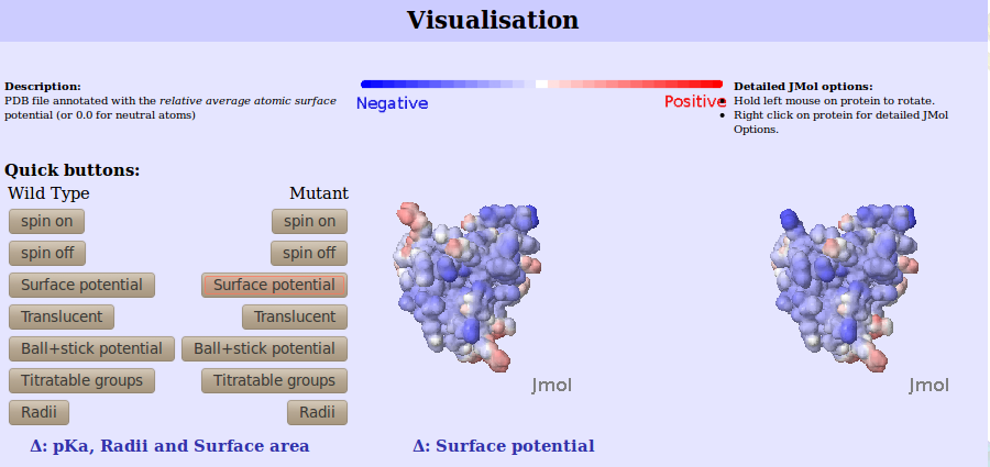 |
| Figure 1. The JMOL interface for the calculated surface potential for both mutant and wild type.
Quick buttons are available
for coloring, movements and molecular representation. However, more detailed options for the JMOL viewer
can be accessed by right clicking the protein. In the residue colored black is the wild type residue to undergo mutation
and it is the replaced residue in the mutant protein.
|
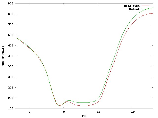
pH-dependant Delta free energy and charge. To complement the surface potential.
Two images/graphs showing the folding free energy and charge of the mutant and wild type proteins,
as they vary against pH, are shown beneath the JMOL visualisation (
these can also be viewed in higher resolution PDF's).
 |
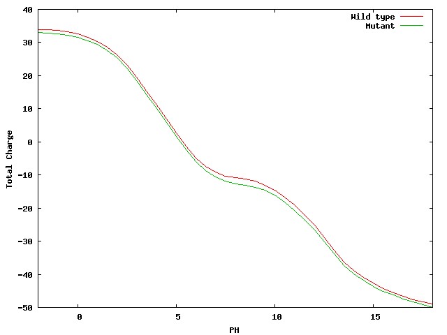 |
| Figure 2. Quick overview of the Delta folding free energy (top) and charge (bottom)
as they vary against the simulated pH for both wild type and mutant protein.
|
Δ pKa, Radii and surface area are calculated by simply subtracting the
wild type values from the mutant values. The information is complimented by distances between the atom and
the mutant. We define this distance to be euclidean distance between the C-β atom of the mutant and
the current atom. It was shown that point mutations more than 15Å from the catalytic site
can affect the activity [11].
Large shifts in pKa between wild type and mutant which are distant in the 3D fold are more
surprising and may indicate possible functionally important residues.
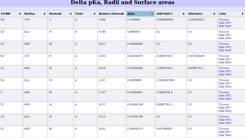 |
| Figure 3. The sorted Δ pKa table. It is sorted by the highest change in
pKa between the wild type and the mutant. In addition, distance information is supplied. For example, atom OH on
residue TYR11 has the largest positive pKa change (0.107) and the distance of this atom to the c-Β atom of the mutated residue
is 4.806 Å.
|
Links to the titration curve and data are also present in this table. These curves show the exact nature of the shift as
a function of pH.
 |
| Figure 4. The titration curve for the basic amino acid Lysine residue 14 (atom NZ).
|
Δ Surface potential. This is simply the subtraction of each atom in the potential calculated in
the wild type from the mutant form. As in the Δ pKa, Radii and surface area table the
information is complimented by distances between the atom and the mutant. Distant changes in surface potential from
the mutated region should be more interesting.
 |
| Figure 5. Potential difference. Sorted by the
difference in potential between the wild type and the mutant. Distance information is also provided.
For example atom 78 HH is 12.816Å from the C-β atom of the mutated residue but yet it has a
sizable change in surface potential (Highest change of 10.6, in positive direction).
|
Sorted tables. There are two sets of tables one for the wild type and one for the mutant.
These are identical to the tables produced when
using bluues on one protein.
|
|
Pymol: how to
|
In order to make the server more useful for experimentalists, the output should be easy to use in PyMol.
The user can download the PDB file, potential for each atom, from the available files and examine the surface potential in pymol using the command promt type:
PyMOL> spectrum b, blue_white_red, minimum=-5, maximum=5
PyMOL> show surface
where -5 and 5 are the min and max potentials and can be modified at will.
In addition, if surface area option is used the PDF file, list of surface points, can also be used within pymol in a similar manner.
|
|
Examples
| |
Below is the link to sample output of the Bluues server. In addition, real biological examples are presented.
Example 1 -
Two exposed amino acid confer thermostability on a mesophilic protein.
This example is taken from [12] where two surface-exposed residues
are responsible for the increase in stability of the thermophilic protein. The two residues are
Arg 3 and Leu 66, in mesophilic proteins both these residues are Glu.
The starting mesophilic protein has PDB code 2ES2A we examine the effect of the
point mutation Glu3Arg.
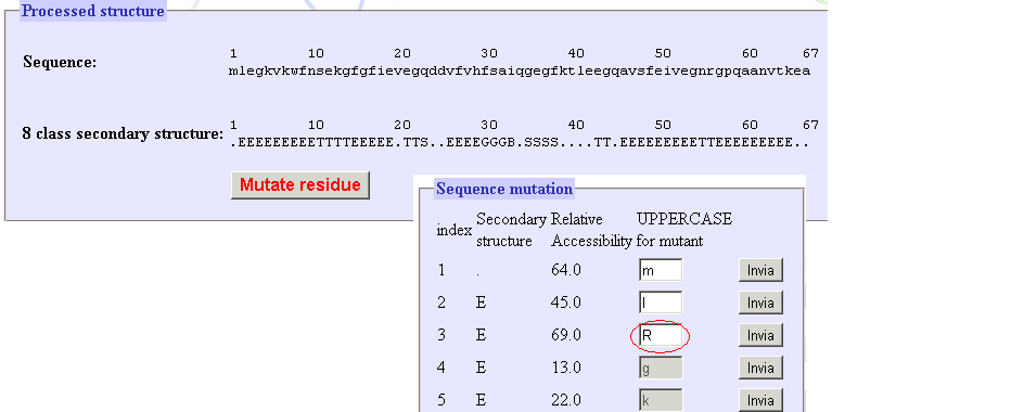 |
| Figure 6. After the PDB is processed its sequence, secondary structure are shown.
A button is available to mutate one residue. The red circle here indicates the point mutation. Point mutations are achieved by
changing the one letter symbol to uppercase. Only residues with relative solvent accessibility above 40% are allowed to be
mutated.
|
The following information was retrieved from the server:
-
The electrostatic Delta free energy changes significantly at pH 4-6 and greater than 8 (approx.).
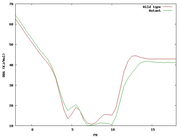 |
| Figure 7. The Delta folding free energy of the wild type and mutant
protein was significantly changed by the mutation.
Glu3Arg.
|
-
The Glu3Arg mutation causes the largest positive pKa change on Glu66 (0.49). Figure 8 shows the exact nature of the change a
titration curve.
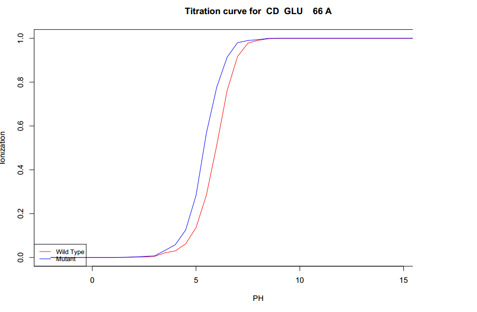 |
| Figure 8. Change in ionization occurs at approximately 3.8 - 8.0.
Glu3Arg.
|
-
Examine the server output yourself and see if you can find other interesting changes. For example, the largest change in
surface potential which is far from the mutated residue.
|
Example 2 -
Tanford transition. The glutamate side chain of residue 89 is buried at pH 6.2 and becomes exposed at
pH 7.1 and 8.2 [13]. For this example,
let us upload two PDB files from TANFORD TRANSITION OF BOVINE BETA-LACTOGLOBULIN: 3BLG solved at pH 6.2 and 2BLG solved at 8.2.
This time we upload the PDB files directly without performing any point mutations.
-
The largest positive pKa change is GLU89 (atom CD) retrieved from the &Delata;pKa table. The change
is 2.663 (positive shift). The exact nature of the change is presented in
figure 9's titration curve. In addition the GB radius change for this atom was 8.595Å.
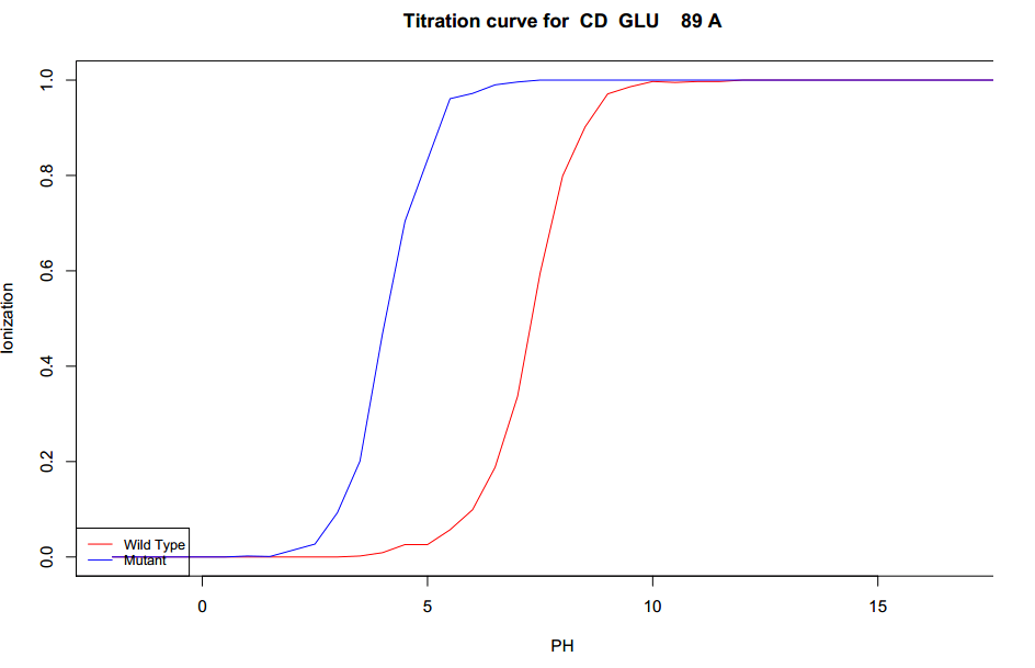 |
| Figure 9. Titration curve for the largest positive changes in pKa.
|
-
The largest negative pKa change is TYR42 (atom OH). The change is -1.476 (negative shift). The exact nature of the change is presented in
figure 10's titration curve. The shift in GB radius was minimal (0.173Å) indicating that this atom does not change conformation.
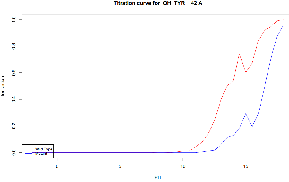 |
| Figure 10. Titration curve for the largest negative changes in pKa.
|
-
Examine the server output yourself and see if you can find other interesting changes.
|
References
|
If you use the server in work leading to publications:
Please cite:
Walsh I, Minervini G, Corazza A, Esposito G, Tosatto S.C.E. and Fogolari F.
Bluues Server: electrostatic properties of wild-type and mutated protein structures.
Bioinformatics. submitted. (2012)
Bluues Method:
Fogolari F, Corazza A, Yarra V, Jalaru A,
Viglino P and Esposito G.
Bluues: a program for the analysis
of the electrostatic properties of proteins
based on generalized Born radii
BMC Bioinformatics in press (2012)
Other references:
-
Fogolari F, Brigo A, Molinari H.
The Poisson-Boltzmann equation for biomolecular electrostatics: a tool for structural biology.
J Mol Recognit. 2002 15:377-92.
-
Dolinsky TJ, Nielsen JE, McCammon JA and Baker NA.
PDB2PQR: an automated pipeline for the setup of Poisson–Boltzmann electrostatics calculations
Nucl. Acids Res. (2004) 32 (suppl 2):W665-W667.
-
Mongan J, Svrcek-Seiler WA and Onufriev A.
Analysis of integral expressions for effective Born radii.
J Chem Phys. 2007 Nov 14;127(18):185101.
-
Tjong H, Zhou HX
GBr6: a parametrization free, accurate, analytical generalized Born method.
J. Phys. Chem. 2007, 111:3055-3061.
-
Grycuk T
Deficiency of the Coulomb-field approximation in the generalized Born model: An improved formula for Born radii evaluation.
J. Chem. Phys. 2003, 119:4817-4826.
-
Antosiewicz J, McCammon JA, Gilson MK
Prediction of pH-dependent properties of proteins.
J. Mol. Biol. 1994, 238:415-436.
-
Schutz CN, Warshel A.
What are the dielectric "constants" of proteins and how to validate electrostatic models?
Proteins. 2001 Sep 1;44(4):400-17.
-
Li H, Robertson AD and Jensen JH.
Very fast empirical prediction and rationalization of protein pKa values.
Proteins 2005, 61:704–721.
-
Rajagopalan PT, Lutz S, Benkovic SJ.
Coupling interactions of distal residues enhance dihydrofolate reductase catalysis: mutational effects on hydride transfer rates.
Biochemistry. 2002 Oct 22;41(42):12618-28.
-
Perl, D., Mueller, U., Heinemann, U., and Schmid, F.X.
Two exposed amino acid residues confer thermostability on a cold shock protein.
Nature Structural Biology 7, 380 - 383 (2000).
-
Qin BY, Bewley MC, Creamer LK, Baker HM, Baker EN, Jameson GB.
Structural basis of the Tanford transition of bovine beta-lactoglobulin.
Biochemistry. 1998 Oct 6;37(40):14014-23.
| |
| | | | | | |